Solvers and examples#
Building NESO with configuration option -DNESO_BUILD_SOLVERS=ON will generate a number of solver executables that can be used to run example simulations.
Note that this option is turned on by default, but is disabled when building NESO via spack with the +libonly variant.
Source code for each solver is in solvers/<solver_name> and input files for the solver examples can be found in examples/<solver_name>.
Note that these examples are intended to demonstrate various features of the NESO library, rather than to simulate particular scenarios of interest in plasma physics.
The solver source codes also act as potential starting points for constructing new applications.
More general instructions for running solvers and modifying example meshes can be found towards the end of this section. The following subsections describe the solvers and accompanying examples that are currently available in NESO.
The Diffusion solver#
Overview#
The Diffusion solver was written by Chris Cantwell and Dave Moxey as a Nektar++ proxyapp for the NEPTUNE project.
The original source code and accompanying documentation can be found in the nektar-diffusion GitHub repository.
The cwipi example is based on another Nektar++ proxyapp, nektar-cwipi.
Equations#
Both the unsteady_aniso and cwipi examples, solve an unsteady, anisotropic (heat) diffusion problem, that is
where \(T\) is the temperature, \(n\) is the number density, \(Q\) is a source term and \(\mathbf{\kappa}_s\) is the anisotropic diffusion tensor.
\(\mathbf{\kappa_s}\) can be decomposed into three orthogonal components; \(\kappa_{\parallel}\), \(\kappa_{\perp}\) and \(\kappa_{\wedge}\):
For a plasma, \(\kappa_{\parallel}\), \(\kappa_{\perp}\) and \(\kappa_{\perp}\) can be identified with Braginskii transport coefficients.
These coefficients are very different for electrons and ions, but considering the regime where B \(\sim 1 T\) and \(T_e~\sim~T_i\), we have \(\kappa_{\parallel} \simeq \kappa_{\parallel}^e\) and \(\kappa_{\perp}\simeq \kappa_{\perp}^i\), such that
and for 2D problems: \(\kappa_{\wedge}^e = \kappa_{\wedge}^i \simeq 0\).
Model parameters#
The table below shows a selection of the model parameters that can be modified in the XML configuration files.
Parameter |
Description |
Reference value |
|---|---|---|
A = m_i/m_p |
Ion mass in proton masses |
1 |
B |
Magnitude of the magnetic field |
1.0 T |
n |
Number density of ions/electrons |
\(10^{18}\) ms \(^{-1}\) |
T |
(Electron) temperature |
116050 K (\(\sim\) 10 eV) |
theta |
Angle between the magnetic field and the x-axis in degrees |
2.0 |
Z |
Ion charge state |
+1 |
lambda |
Coulomb logarithm |
13 |
TimeStep |
Time step size |
0.001 |
NumSteps |
Total number of time steps |
5 |
IO_CheckSteps |
Number of time steps between outputs |
1 |
Implementation#
In both examples, the anisotropic diffusion problem is solved on a square mesh of 80x80 quads using a Continuous Galerkin discretisation.
The initial conditions have a top-hat like profile on the left edge of the domain:
The systems are solved using a Conjugate Gradient method and a simple Diagonal preconditioner. Timestepping is performed with a first-order BDF method.
Examples#
unsteady_aniso#
Configuration files for the unsteady_aniso example can be found in examples/Diffusion/unsteady_aniso.
The Gmsh file, square.geo, file is supplied in case users wish to modify the mesh, but the simulations only requires the xml files to run.
The easiest way to execute the example is with
./scripts/run_eg.sh Diffusion unsteady_aniso
which makes a copy of the example directory and executes the Diffusion solver in that location, using the command in examples/Diffusion/unsteady_aniso/run_cmd_template.txt.
cwipi#
N.B. To run the `cwipi` example, NESO must be built with configuration option -DNESO_BUILD_CWIPI_EXAMPLES=ON and Nektar++ must have been built with option -DNEKTAR_USE_CWIPI=ON.
The easiest way to enable all required options is to build the 'cwipi' variant of NESO via spack; i.e. spack install neso+cwipi
Configuration files for the cwipi example can be found in examples/Diffusion/cwipi.
Like the previous example, an unsteady anisotropic diffusion problem is solved.
Unlike the previous example, the process is split into two tasks, performed by separate executables and coupled via the CWIPI framework.
The first executable computes the diffusion tensor based on the parameters set in its configuration file.
This tensor is then sent, via MPI, to the second executable, which uses it to evolve the system from the initial conditions and generate a solution.
Each executable can itself run using multiple MPI processes.
The MPI command used to run the coupled problem can be found in examples/Diffusion/cwipi/run_cmd_template.txt, but the easiest way to execute the example is:
./scripts/run_eg.sh Diffusion cwipi

N.B. The Diffusion solver occasionally hangs during the initialisation stage when running the `cwipi` example.
Rerunning the command above should work around the issue.
While this example is somewhat artificial, it serves to demonstrate how Nektar++, via CWIPI can be used to couple independent executables. Other possible applications include running solvers in neighbouring domains and coupling them via boundary conditions with each domain representing a different material. This could be used to model, for example, plasma turbulence in the tokamak edge and the resulting heat diffusion into the first wall.
Outputs#
Outputs from the solver are written as Nektar++ checkpoint (.chk) files.
The easiest way to visualise them is to convert them to vtu format and inspect them in Paraview.
The final state of both examples should look like this:
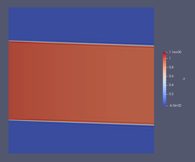
Temperature field (labelled ‘u’) in the final output of the unsteady_aniso example.
The DriftPlane solver#
Overview#
The DriftPlane solver is based on a Nektar++ proxyapp written by Dave Moxey for the NEPTUNE project.
The original source code and accompanying documentation can be found in the nektar-driftplane GitHub repository.
Examples#
blob2D#
The blob2D example was inspired by the BOUT++/Hermes-3 demo of the same name. It tracks the formation of a plasma filament from an overdense “blob”, subject to a diamagnetic drift force.
The model considers a single, isothermal fluid evolving in a square domain where the x-axis represents the radial coordinate in a tokamak and the \((x,y)\) plane is a 2D slice at a particular toroidal angle. Moving to the right through the domain corresponds to moving further towards the outboard side of the tokamak.
Equations#
The equations are:
where \(n\) is the electron density, \(\omega\) is the electron vorticity and \(\phi\) is the electrostatic potential. \(\epsilon\frac{\partial n_e}{\partial y}\) is the diamagnetic drift term. \(\frac{n_e \phi}{L_{\parallel}}\) is a “connection term” that stands in for the divergence of the sheath current, \(\nabla \cdot {\bf j}_{sh}\), in order to capture the behaviour of the plasma at the ends of the field lines, perpendicular to the simulation domain (the drift-plane). \(L_{\parallel}\) is the connection length.
A more detailed discussion of the model can be found in section 2.1 of the M6c.3 project NEPTUNE report.
Model parameters#
The table below shows a selection of the configuration options that can be modified under the PARAMETERS node of the blob2d XML configuration file.
Parameter |
Label in config file |
Description |
Default Value |
|---|---|---|---|
\(B\) |
B |
(Poloidal) magnetic field strength in T. |
0.35 |
\(T_{e0}\) |
T_e |
Electron temperature in eV. |
5 |
\(L_\parallel\) |
Lpar |
Connection length in m. |
10.0 |
\(R_{xy}\) |
Rxy |
Tokamak major radius in m. |
1.5 |
init_blob_norm |
(Density) amplitude of initial Gaussian blob. |
0.5 |
|
init_blob_width |
Width of initial Gaussian blob in m. |
0.05 |
Note that the factor \(\epsilon\) in the vorticity equation is calculated by the code internally as \(\epsilon=\frac{e T_e}{R_{xy}^2}\).
Implementation#
In the DriftPlane solver, the blob2D system is discretised using a Discontinous Galerkin formulation for the density and vorticity and Continuous Galerkin for the potential. The potential is not evolved directly, but is calculated at each timestep from the the vorticity using Nektar++’s Helmholtz solver. The mesh is a unit square of 64x64 quadrilateral elements and 5th order basis functions are used for all fields. The initial density condition is a Gaussian blob at the centre of the domain, while the vorticity (and therefore the potential) is set to zero everywhere. Nektar++’s default solver options are used, that is, a Conjugate Gradient method with static condensation and a simple Diagonal/Jacobi preconditioner. Timestepping is performed with a 4th order Runge-Kutta (explicit) method.
Output#
Field outputs from the solver are written as Nektar++ checkpoint (.chk) files.
The easiest way to visualise them is to convert them to vtu format and inspect them in Paraview.
Evolution of the electron density should resememble the images shown below.
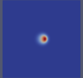
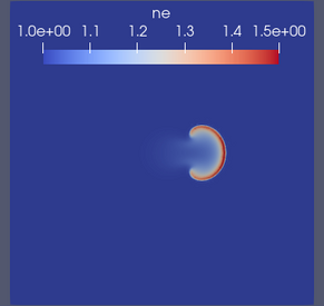
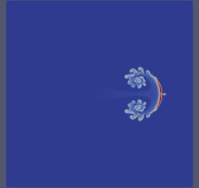
Electron density at t=0.4 (left), t=1.2 (centre) and t=2 (right) in the blob2D example.
The DriftReduced solver#
Overview#
The DriftReduced solver provides a number of simple models for 2D and 3D plasma turbulence.
All of these models either directly or indirectly incorporate an \(E{\times}B\) plasma drift velocity, calculated via the gradient of the electrostatic potential, which in turn is calculated from a vorticity field. The machinery to compute the drift velocity, and then advect the plasma accordingly, is therefore implemented in a common class from which all of the DriftReduced model equation systems are derived.
The following subsections describe the examples that are currently available.
Note that many of the DriftReduced examples are expected to exhibit chaotic behaviour, with small numerical differences between compilers and platforms being magnified over the course of a simulation.
While the statistical properties of fluid fields are expected to be robust, outputs may differ in detail from those shown.
Examples#
2DHW#
The 2DHW equation system and example are adapted from a Nektar++ proxyapp written by Dave Moxey and Jacques Xing for the NEPTUNE project.
The original source code and accompanying documentation can be found in the nektar-driftwave GitHub repository.
The example can be run with
./scripts/run_eg.sh DriftReduced 2DHW
Equations#
Solves the 2D Hasegawa-Wakatani (HW) equations. That is:
where \(\omega\) is vorticity and \(\phi\) is the electrostatic potential. The potential can be obtained from the vorticity by solving the Possion equation \(\nabla^2\omega = \phi\). \(n\) is plasma number density relative to a fixed background profile, so need not be positive. The background profile is assumed to be exponential with a scale length related to \(\kappa\). The strength of the coupling between the density and the potential is mediated by \(\alpha\), the adiabacity parameter.
\([a,b]\) is the Poisson bracket operator, defined as
Note that equations (1) and (2) represent the “unmodified” form of the HW equations, which don’t include so-called zonal flows (see e.g. this webpage for further explanation.)
HW Model parameters#
The table below shows a selection of the configuration options that can be modified under the PARAMETERS node of the XML configuration file.
Parameter |
Label in config file |
Description |
Default value |
|---|---|---|---|
\(B\) |
Bxy |
Magnetic field strength (normalised units) |
1.0 |
\(\alpha\) |
HW_alpha |
Adiabacity parameter: controls coupling between \(n\) and \(\phi\) |
2.0 |
\(\kappa\) |
HW_kappa |
Turbulent drive parameter: assumed scale length of background exponential density profile |
1.0 |
- |
s |
Initial blob size: Scale length of the Gaussian density ICs (normalised units) |
2.0 |
Table 1: Configurable model parameters for the 2DHW example
Implementation#
The 2DHW system is discretised using a Discontinous Galerkin formulation for the density and vorticity and Continuous Galerkin for the potential.
The potential is not evolved directly, but is calculated at each timestep from the the vorticity using Nektar++’s Helmholtz solver.
The use of DG for the time-evolved fields increases stability sufficiently that it isn’t necessary to include the hyperdiffusivity terms (\(\mu \nabla^4 n\), \(\mu \nabla^4 \omega\)) that are often added to other HW implementations.
The mesh is a 20x20 square of 64x64 quadrilateral elements and 3rd order basis functions are used for all fields.
Boundary conditions are periodic in both the \(x\) and \(y\) dimensions for all fields.
The initial conditions for density and vorticity are Gaussians with widths \(s\) (see Table 1):
Nektar++’s default solver options are used, that is, a Conjugate Gradient method with static condensation and a simple Diagonal/Jacobi preconditioner. Timestepping is performed with a 4th order Runge-Kutta (explicit) method.
Outputs#
Processing the final checkpoint of the simulation and rendering it in Paraview should produce output resembling the images below:
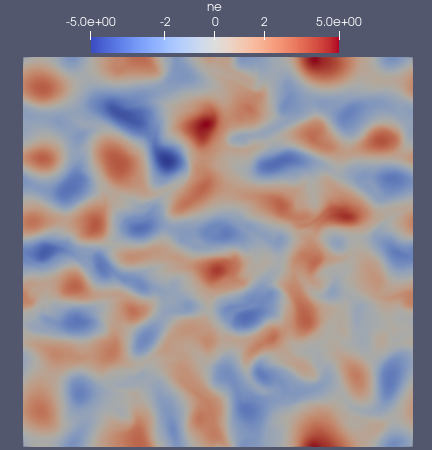
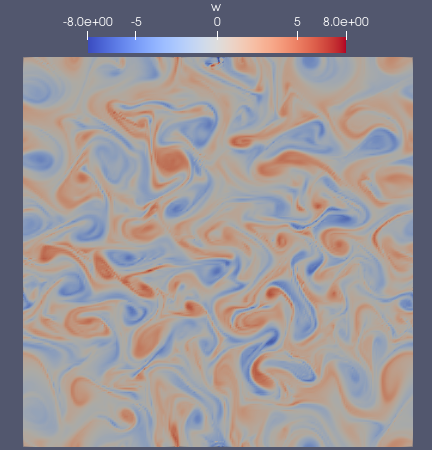
Density (left) and vorticity (right) in the final output of the 2DHW example (t=50).
2Din3DHW_fluid_only#
Solves the 2D HW equations, (1) and (2), in a 3D domain. The magnetic field is assumed to be constant and parallel to the z-axis, so that the Poisson solve for the potential becomes
where the \(_\perp\) subscript denotes the restriction of the Laplacian to the two-dimensional subspace transverse to the field lines.
More details of the implementation can be found in section 2.3.1 of NEPTUNE report M4c.3.
The example can be run with
./scripts/run_eg.sh DriftReduced 2Din3DHW_fluid_only
Implementation#
The list of configurable model parameters is the same as for the 2DHW example; see Table 1.
The domain is a cuboid with dimensions (arbitrary length units) 5x5x10.
The mesh, generated via Gmsh and Nekmesh, has 8x8x16 hexahedral elements and 6th order basis functions are used for all fields.
Boundary conditions are periodic in all three dimensions.
Nektar++’s default solver options are used, that is, a Conjugate Gradient method with static condensation and a simple Diagonal/Jacobi preconditioner.
Timestepping is performed with a 4th order Runge-Kutta (explicit) method.
Although all of the modelled dynamics are in the (x,y) subspace, variation is introduced in the z dimension by modulating the initial conditions used in the 2DHW example with a sinusoidal function in the \(z\) direction:
Outputs#
Field outputs from the solver are written as Nektar++ checkpoint (.chk) files.
The easiest way to visualise them is to convert them to vtu format and inspect them in Paraview.
Evolution of the electron density should resememble the images shown below.
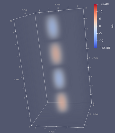
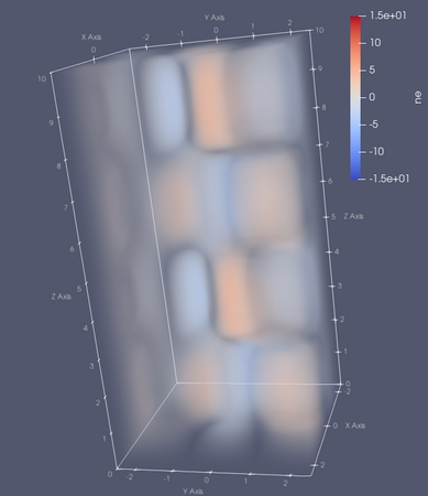
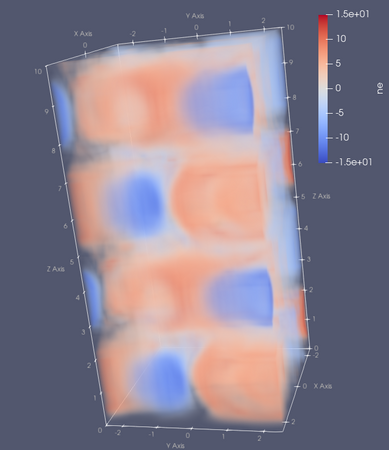
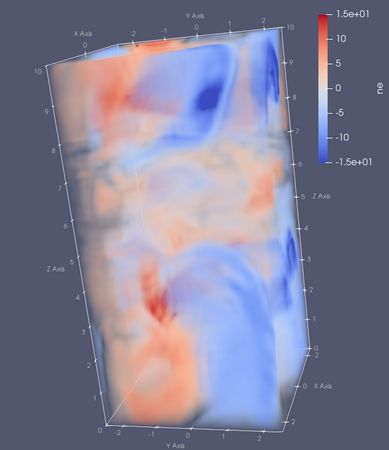
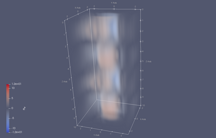
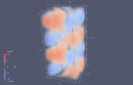
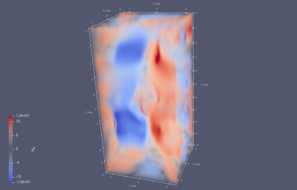
Electron density at t=0 (top-left), t=12.5 (top-right), t=25 (bottom-left) and t=40 (bottom-right) in the 2Din3DHW_fluid_only example
2Din3DHW#
The fluid model and equations considered in the 2Din3DHW example are the same as those described above.
Equations (1) and (2) are solved in a 3D domain, but additional source terms from (Hydrogenic) ionisation are added by including a system of kinetic neutrals that are coupled to the fluid solver.
The example can be run with
./scripts/run_eg.sh DriftReduced 2Din3DHW
Model parameters#
In addition to those parameters listed in Table 1, a number of particle system properties can be configured.
Parameter |
Label in config file |
Description |
Default value |
|---|---|---|---|
\(N_{\rm part}\) |
num_particles_total |
Total number of (neutral) particles to generate. |
100000 |
\(n_{\rm phys}\) |
particle_number_density |
Physical number density of neutrals in SI units |
1e16 |
\(v_{\rm th}\) |
particle_thermal_velocity |
Width of the Gaussian from which random particle thermal velocities are drawn. Normalised units. |
1.0 |
\(v_{\rm d}\) |
particle_drift_velocity |
Bulk drift velocity given to all particles. Normalised units. |
2.0 |
\(\sigma_p\) |
particle_source_width |
Width of the Gaussian from which random particle positions are drawn. Normalised units. |
0.2 |
\(T\) |
Te_eV |
Assumed electron temperature in eV. |
10.0 |
Table 2: Configurable model parameters for the 2Din3DHW example
Implementation#
The domain, mesh, fluid solver properties and boundary conditions in this example are the same as those described in the 2Din3DHW_fluid_only example.
The initial conditions are set to zero throughout the domain for both \(n\) and \(\omega\), such that all non-trivial evolution of the fluid fields is triggered by particle sources.
Neutral particles, like the fluid fields, are subject to periodic boundary conditions in all three dimensions.
\(N_{\rm part}\) computational particles are generated at the beginning of the simulation and assigned initial weights (equal to the number of physical neutrals that they represent) such that the overall number density in the domain matches the requested \(n_{\rm phys}\) value.
Initial particle positions are chosen by drawing values at random from a 3D Gaussian distribution centred at the origin and with a width \(\sigma_p\). Initial velocities are assigned a bulk drift velocity, \(v_{\rm d}\), which is added to a random thermal velocity, drawn from a second Gaussian of width \(v_{\rm th}\).
At every particle timestep, the fluid density is evaluated at each computational particle position and used, in combination with the assumed temperature, to compute the rate at which neutral Hydrogen atoms are expected to be ionised (\(r_{\rm ionise}\)) according to equation 5 in Lotz, 1968.
The computational particle weight is then reduced by an amount
where \(w_i\) is the current weight associated with each particle, \(n\) is the (fluid) number density evaluated at its position and dt is the length of the time step.
More details of the implementation can be found in section 2.3.1 of NEPTUNE report M4c.3.
Outputs#
Fluid field outputs from the solver are written as Nektar++ checkpoint (.chk) files and all particle data is written to DriftReduced_particle_trajectory.h5part.
Both can be visualised together by converting the checkpoint files to vtu format and then loading both the .vtu files and the .h5part file in Paraview.
The early evolution of the plasma density and the neutral particle weights should resememble the images shown below.
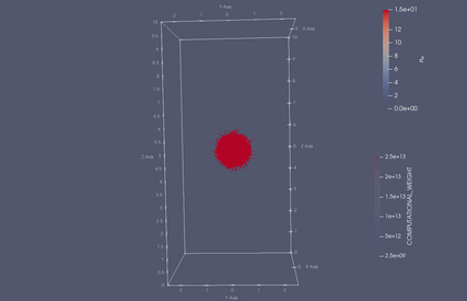
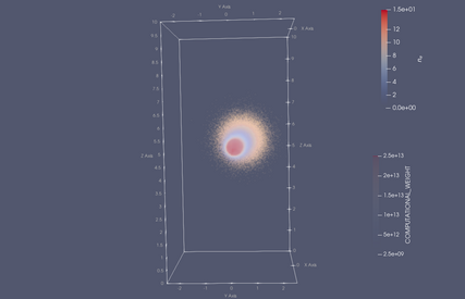
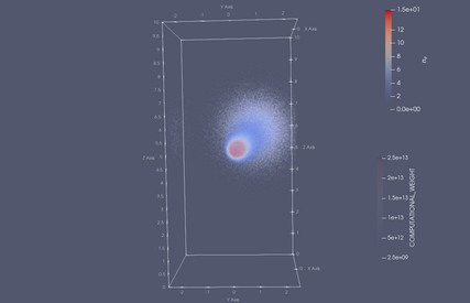
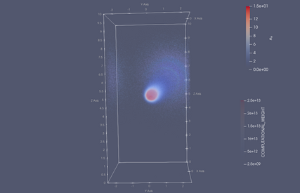
Evolution of the particle distribution (points) and electron density (coloured contours) during the early part of the 2Din3DHW example.
Particles are coloured according to their computational weight, corresponding to the number of physical neutrals that they represent.
Output times are t=0 (top-left), t=0.225 (top-right), t=0.45 (bottom-left) and t=0.675 (bottom-right).
The particles start in a Gaussian blob with a bulk drift, before spreading out due to variations in their thermal velocities. As the simulation progresses, neutral particles ionise, reducing the weight associated with each computational particle (blue points) and adding to the plasma density (redder contours).
2DRogersRicci#
Model based on the 2D (finite difference) implementation described in “Low-frequency turbulence in a linear magnetized plasma”, B.N. Rogers and P. Ricci, PRL 104, 225002, 2010 (link); see their equations (7)-(9).
The example can be run with
./scripts/run_eg.sh DriftReduced 2DRogersRicci
Equations#
In SI units, the equations are:
where
and the source terms have the form
where \(r = \sqrt{x^2 + y^2}\)
Model parameters#
Parameter |
Label in config file |
Description |
Default Value |
|---|---|---|---|
\(T_{e0}\) |
T_0 |
Temperature. |
6 eV |
\(m_i\) |
m_i |
Ion mass. |
6.67e-27 kg |
\(\Lambda\) |
coulomb_log |
Couloumb Logarithm. |
3 |
\(\Omega_{ci}\) |
Omega_ci |
Ion cyclotron frequenxy in Hz. |
\(9.6e5\) |
R |
R |
Approx. radius of the plasma column. |
0.5 m |
Table 3: Configurable model parameters for the 2DRogersRicci example
Derived values
Parameter |
Description |
Calculated as |
Value |
|---|---|---|---|
B |
Magnetic field strength. |
\(\Omega_{ci} m_i q_E\) |
40 mT |
\(c_{s0}\) |
Sound speed. |
\(\sqrt{T_{e0}/m_i}\) |
1.2e4 ms-1 |
\(\rho_{s0}\) |
Larmor radius. |
\(c_{s0}/\Omega{ci}\) |
1.2e-2 m |
\(S_{0n}\) |
Density source scaling factor. |
0.03 \(n_0 c_{s0}/R\) |
4.8e22 m-3s-1 |
\(S_{0T}\) |
Temperature source scaling factor. |
0.03 \(T_{e0} c_{s0} / R\) |
4318.4 Ks-1 |
\(\sigma\) |
\(1.5 R/L_z\) |
1/24 |
|
\(L_s\) |
Scale length of source terms. |
\(0.5\rho_{s0}\) |
6e-3 m |
\(r_s\) |
Approx. radius of the LAPD plasma chamber. |
\(20\rho_{s0}\) |
0.24 m |
Normalisation#
Normalisations follow those in Rogers & Ricci, that is:
Normalised to |
|
|---|---|
Charge |
\(e\) |
Electric potential |
\(e/T_{e0}\) |
Energy |
\(T_{e0}\) |
Number densities |
\(n_0\) |
Perpendicular lengths |
\(100 \rho_{s0}\) |
Parallel lengths |
\(R\) |
Time |
\(R/c_{S0}\) |
The normalised forms of the equations are:
with
where \(\rho_{s0}\), \(r_s\) and \(Ls\) have the (SI) values listed in the tables above.
Implementation#
The default initial conditions are
Field |
Default ICs (uniform) |
|---|---|
n |
\(2\times10^{14}\) \({\rm m}^{-3}\) (\(10^{-4}\) normalised) |
T |
\(6\times10^{-4}\) eV (\(10^{-4}\) normalised) |
\(\omega\) |
0 |
All fields have Dirichlet boundary conditions with the following values:
Field |
Dirichlet BC value |
|---|---|
n |
\(10^{-4}\) |
T |
\(10^{-4}\) |
\(\omega\) |
0 |
\(\phi\) |
\(\phi_{\rm bdy}\) |
\(\phi_{\rm bdy}\) is set to 0.03 by default. This value ensures that \(\phi\) remains relatively flat outside the central source region and avoids boundary layers forming in \(\omega\) and \(\phi\).
The mesh is a square with the origin at the centre and size \(\sqrt{T_{e0}/m_i}/\Omega{ci} = 100\rho_{s0} = 1.2\) m. By default, there are 64x64 quadrilateral (square) elements, giving sizes of 1.875 cm = 25/16 \(\rho_{s0}\) The default simulation time is \(\sim 12\) in normalised units (= \(500~{\rm{\mu}s}\)).
Outputs#
Processing the final checkpoint of the simulation and rendering it in Paraview should produce output resembling the image below:
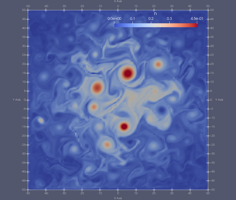
Density in normalised units, run with the implicit DG implementation on a 64x64 quad mesh for 12 normalised time units (5 ms).
3DHW#
Solves the 3D HW equations in a slab geometry with a fixed, axis-aligned magnetic field.
The example can be run with
./scripts/run_eg.sh DriftReduced 3DHW
Equations#
The 3D Hasegawa-Wakatani equations are similar to the 2D equations, but with the constant adiabacity parameter replaced by a second order spatial derivative in the parallel direction, that is:
Note that, as with the 2D HW equations, (1) and (2), \(n\) represents a fluctuation on a fixed background. Computing \(\phi\) at each timestep takes place in exactly the same way as described in the 2Din3DHW_fluid_only example.
Model parameters#
The values of \(\alpha\) and \(\kappa\) may be set in the same way as the other HW examples (see labels in Table 1). Note that \(\alpha\) has a slightly different meaning in the 2D and 3D version of the equations. The following additional parameters can be set in 3D as an alternative to specifying \(\alpha\) and \(\kappa\) directly:
Parameter |
Label in config file |
Description |
Default value |
|---|---|---|---|
\(m_i\) |
mi |
Ion mass in kg. |
2 \(\times\) 1.67 \(\times 10^{-27}\) kg |
\(n_0\) |
n0 |
Background density in \({\rm m}^{-3}\). |
None |
\(T_0\) |
T0 |
Background temperature in eV. |
None |
\(Z\) |
Z |
Ion charge state. |
None |
\(\lambda_n\) |
lambda_q |
Scrape-off layer density width in m. |
None |
If all of the parameters, \(m_i\), \(n_0\), \(T_0\) and \(Z\) are provided, they will be used to calculate a value for \(\alpha\) via:
where \(\eta\) is the Spitzer electron resistivity and \(\omega_{ci}\) is the ion cyclotron frequency.
If all of the parameters, \(m_i\), \(n_0\), \(T_0\) and \(\lambda_n\) are provided, they will be used to calculate a value for \(\kappa\) via:
where \(\rho_{s0}\) is the the ion gyro-radius.
Implementation#
Like the other Hasegawa-Wakatani examples, the 3DHW system is discretised using a Discontinous Galerkin formulation for the density and vorticity and Continuous Galerkin for the potential, and the potential is calculated via equation 3 using Nektar++’s Helmholtz solver.
The domain is a cuboid shape which is twice as long in the field-parallel direction as in normal and bi-normal directions. (dimensions 5x5x10).
Fluid elements are unit cubes and 6th order basis functions are used for all fields.
The initial conditions for \(\phi\) and \(n\) are the same as those used in the 2Din3DHW_fluid_only (see equations 4 and 5)
Boundary conditions for all fields are periodic in all three dimensions.
Nektar++’s default solver options are used, that is, a Conjugate Gradient method with static condensation and a simple Diagonal/Jacobi preconditioner. Timestepping is performed with a 4th order Runge-Kutta (explicit) method.
Outputs#
Outputs from the example are written as Nektar++ checkpoint (.chk) files.
The easiest way to visualise the fields is to convert the files to vtu format and inspect them in Paraview.
Evolution of the electron density should resememble the images shown below.
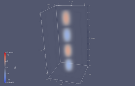
Evolution of the electron density in the 3DHW example.
Output times are t=0 (top-left), t=10 (top-right), t=25 (bottom-left) and t=40 (bottom-right).
Diagnostics#
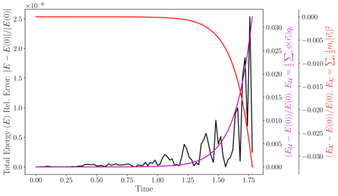
For the Hasegawa-Wakatani examples (2DHW, 2Din3DHW_fluid_only, 2Din3DHW, 3DHW), the solver can be made to output the total fluid energy (\(E\)) and enstrophy (\(W\)), which are defined as:
In the 2DHW and 2Din3DHW_fluid_only examples, the expected growth rates of \(E\) and \(W\) can be calculated analytically according to:
where
To change the frequency of this output, modify the value of growth_rates_recording_step inside the <PARAMETERS> node in the example’s configuration file.
When that parameter is set, the values of \(E\) and \(W\) are written to <run_directory>/growth_rates.h5 at each simulation step \(^*\). Expected values of \(\frac{dE}{dt}\) and \(\frac{dW}{dt}\), calculated with equations (15) and (16) are also written to file, but note that these are only meaningful when particle coupling is disabled.
\(^*\) Note that the file will appear empty until the file handle is closed at the end of simulation.
The Electrostatic2D3V solver#
Overview#
The theory behind the Electrostatic2D3V solver and the two_stream example can be found in NEPTUNE report M4c.1: 1-D and 2-D Particle Models; see section 2.2 in particular.
Examples#
two_stream#
The example can be run with
./scripts/run_eg.sh Electrostatic2D3V two_stream
Outputs and postprocessing#
Unlike other NESO examples, the Electrostatic2D3V solver doesn’t generate Nektar++ checkpoint files.
Instead it outputs Electrostatic2D3V_field_trajectory.h5 which contains particle data in H5Part format, a derivative of HDF5.
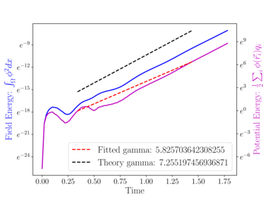
This file can be visualised in (e.g.) Paraview or postprocessed using the supplied Python script, which plots the energy evolution and compares it to theory.
To run the script, install all required Python packages, then pass it the Nektar++ configuration file and the .h5 file as arguments:
pip install -r requirements.txt
python3 plot_two_stream_energy.py two_stream.xml Electrostatic2D3V_field_trajectory.h5
The plots are written to field_energy.pdf and all_energy.pdf and are reproduced below for convenience:
The SimpleSOL solver#
The SimpleSOL solver models transport along a field line in the scrape-off layer (SOL) of a tokamak.
The domain is a symmetric flux tube, wherein plasma is assumed to enter from the perpendicular direction due to cross-field transport, then move along the field line towards a divertor (at both ends).
At the divertor, it is assumed that plasma is extracted at a prescribed, constant velocity.
The model describes the evolution of plasma density, velocity and temperature.
Profiles of the three fields when the system has reached a steady state are determined purely by the boundary conditions and the shape of the source terms.
The plasma is assumed to have an ideal gas equation of state.
The solver can also be extended to evolve a system of neutral particles, which ionise and contribute additional source terms to the fluid equations.
Examples#
1D#
The example can be run with
./scripts/run_eg.sh SimpleSOL 1D
Equations#
The equations associated with the 1D SimpleSOL problem are:
where \(s\) is the spatial coordinate \(n\) is the plasma density, \(u\) the plasma velocity, and \(T\) the plasma temperature. \(S^n\), \(S^u\) and \(S_T\) are source terms in density, momentum and temperature respectively. \(g\) is related to the ratio of specific heats, \(\gamma\), by \(g=\frac{2\gamma}{\gamma-1}\) Using the ideal gas law, it can be shown that this system is almost exactly equivalent to the compressible Euler equations. Reframing in that context, (3) becomes an energy equation:
Model parameters#
The model parameters in the SimpleSOL solver are mostly used to set the boundary conditions and (Gaussian) source widths.
The table below shows a selection of the configuration options that can be modified under the PARAMETERS node of the XML configuration file.
Parameter |
Label in config file |
Description |
Reference value |
|---|---|---|---|
\(\gamma\) |
Gamma |
Ratio of specific heats |
5/3 |
\(P_{\rm inf}\) |
pInf |
Downstream pressure. |
1.0 |
\(n_{\rm inf}\) |
rhoInf |
Downstream density. |
1.0 |
\(u_{\rm inf}\) |
uInf |
Downstream velocity. |
1.0 |
\(\sigma_s\) |
srcs_sigma |
Width of fluid source terms |
2.0 |
Implementation#
The similarity between the SimpleSOL equation system and the compressible Euler equations means that elements of Nektar++’s CompressibleFlowSolver can be used to evolve the fluid fields. This casts the equations in conservative form; see section 9.1.1 in the Nektar++ user guide for further discussion.
The domain is a line of length 110 units, divided into 56 segments.
9th order basis functions are used for each segment/element.
We note that such a high order appears to be required in this example due to the relatively sharp fluid sources and the lack of diffusive terms in the equations.
\(n\), \(nu\) and \(E\) are discretised using a Discontinuous Galerkin approach.
Upwinding is added using Nektar++’s built-in ExactToro Riemann solver.
All fields are initialised to constant values across the domain: \(n=n_{\rm inf}\), \(nu=0\) and \(E=P_{\rm inf}/(\gamma-1)\).
The (Dirichlet) boundary conditions at the ends of the flux tube are
where outflow boundary conditions are enforced by setting \(\alpha=-1\) at one end of the domain, and \(1\) at the other.
Nektar++’s default solver options are used, that is, a Conjugate Gradient method with static condensation and a simple Diagonal/Jacobi preconditioner. Timestepping is performed with a 4th order Runge-Kutta (explicit) method.
Outputs#
Field outputs from the solver are written as Nektar++ checkpoint (.chk) files.
One way to postprocess the data is to convert those files to vtu format and apply Filters in Paraview.
Another way is to use the NekPy Python package to read the outputs directly.
The image below shows the result of extracting field data from the final snapshot, using NekPy, and postprocessing it to compute \(n\), \(u\) and \(T\) profiles. These profiles may then be compared to the analytic solutions for the appropriate set of source terms:
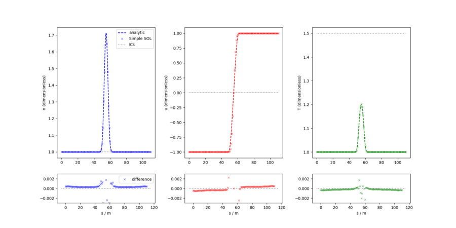
Comparison between the steady state profiles of n, u and T and the analytic steady state solutions. Bottom panels show the residual between the simulated and analytic profiles.
2D#
The 2D version of the (inherently 1D) SimpleSOL model imagines that the flux tube has a small but non-zero width. In this case, the fluid source terms have a constant value in the cross-field direction, and the same profiles as before in the field-parallel direction. This implementation was originally added as a test of neutral particle coupling (see the next example).
The example can be run with
./scripts/run_eg.sh SimpleSOL 2D
Equations#
Taking equations 1, 2 and 4 and generalising to more than one dimension, we have:
where \(\vec{I}\) is the identity matrix.
Model parameters#
In 2D, the direction of the field line is always assumed to be parallel to the long side of the rectangular domain, although this need not be aligned with the x coordinate axis. If the domain is rotated (by providing a new mesh file), the source terms need to be adjusted by specifying \(\theta\), the angle between the field line and the horizontal. The length of the domain is not calculated automatically by the code and also needs to be supplied via the \(L_s\) parameter.
Parameter |
Label in config file |
Description |
Reference value |
|---|---|---|---|
\(\theta\) |
theta |
Angle (in radians) between the field line/flow axis and the x-axis. |
0.0 |
\(L_s\) |
unrotated_x_max |
Domain length (ignoring rotation). |
110.0 |
Implementation#
The 2D system is implemented in the same way as the 1D system, with additional (scalar) DG field for the cross-field momentum.
The mesh is a 110x1 rectangle of 110x3 quadrilateral elements. 4th order basis functions are used for all fields.
Boundary conditions are periodic in the cross-field direction and (Dirichlet) at the ends of the flux tube, using the same values set in the 1D example.
All fields are initialised to constant values across the domain: \(n=n_{\rm inf}\), \(nu=nv0\) and \(E=P_{\rm inf}/(\gamma-1)\).
Nektar++’s default solver options are used, that is, a Conjugate Gradient method with static condensation and a simple Diagonal/Jacobi preconditioner. Timestepping is performed with a 4th order Runge-Kutta (explicit) method.
Outputs#
Outputs are the same as those in the 1D example and can be postprocessed in a similar way.
In order to compare to analytic expectations, profiles should be exctracted along a line parallel to the long axis of the domain, accounting for the value of the \(\theta\) parameter.
2D_with_particles#
In this example,the fluid equations solved are the same as those in the 2D case, but in addition to the plasma fluid, a system of kinetic neutrals is enabled.
The neutral particles undergo ionisation, despositing density, momentum and energy into the plasma.
The example can be run with
./scripts/run_eg.sh SimpleSOL 2D_with_particles
Model parameters#
In addition to the parameters associated with the plasma fluid (see the 1D and 2D examples above), the following configuration options are available for the neutral particle system.
Parameter |
Label in config file |
Description |
Reference value |
|---|---|---|---|
\(N_p\) |
num_particles_total |
Total number of particles (per MPI rank) to add each timestep |
100 |
\(n_N\) |
particle_number_density |
Mean density of physical neutrals added at each timestep |
3e18 |
\(N_{\rm reg}\) |
particle_source_region_count |
Number of particle source regions to generate. Valid values are 1 or 2. |
2 |
\(\delta_{\rm r}\) |
particle_source_region_offset |
Offset between the domain ends and the first/last particles source centres. |
0.2 |
\(N_{\rm bins}\) |
particle_source_line_bin_count |
Number of position bins along the line (cross-field direction). |
4000 |
\(\sigma\) |
particle_source_region_gaussian_width |
Width of the Gaussian particle sources in units of domain length. |
0.001 |
\(N_{\rm l}\) |
particle_source_lines_per_gaussian |
Number of lines that make up each Gaussian source. |
7 |
\(T_{\rm th}\) |
particle_thermal_velocity |
Width of the Gaussian used to draw random thermal velocities. |
1.0 |
\(L_t\) |
unrotated_y_max |
Domain width (ignoring rotation). |
1.0 |
Implementation#
The domain, mesh and fluid solver properties are the same as those used in the 2D example.
Particle neutrals are configured as follows.
With the default value of \(N_{\rm reg}=2\), particles are generated at both ends of the domain, mimicking injection of neutrals near the divertor, or perhaps recycling of neutral particles in the divertor region. Particles are given initial positions along straight lines in the y direction. The two collections of line are centred at \(x=\delta_{\rm r}\) and \(x=L_s-\delta_{\rm r}\). Within each collection, there are \(N_{\rm l}\) source lines with Gaussian spacings around the collection centre. Along each line, positions are drawn uniformly from \(N_{\rm bins}\) bins. Finally, random velocities are assigned to each particle by drawing values from a Gaussian of width \(T_{\rm th}\).
At each timestep, \(N_p\) new computational particles are added by each MPI rank, shared between \(N_{\rm l}\) source lines. Their weights are assigned such that the mean physical neutral density added is \(n_N\).
In the \(y\) direction (perpendicular to the field lines), periodic boundary conditions are imposed on all particles. In the \(x\) direction, particles are tagged for removal if they cross the domain boundary. At the end of each particle step, these tagged particles are deleted from the simulation.
Ionisation rates are a function of plasma temperature, evaluated at the location of each computational particle. Coupling to the fluid solver is achieved by projecting particle properties onto dedicated Nektar++ fields, which are then added as source terms to the density, momentum and energy equations.
More details of the implementation can be found in sections 2.2.4 and 2.2.5 of NEPTUNE report M4c.2.
Outputs#
Fluid field outputs from the solver are written as Nektar++ checkpoint (.chk) files and all particle data is written to SimpleSOL_particle_trajectory.h5part.
Both can be visualised together by converting the checkpoint files to vtu format and then loading both the .vtu files and the .h5part file in Paraview.
The image below shows the distribution of fluid plasma (upper panel) and neutral particles (lower panel) towards one end of the domain, corresponding to the region closest to the divertor. The position of the particle source centre in the lower panel is easily identified by the concentration of points with high computational weights (redder colours). As the simulation evolves, computational particles move away from the source locations, becoming progressively more ionised (bluer colours) and depositing material onto the plasma density field (redder colours in the upper panel). This is then advected towards the domain boundaries by the fluid solver.
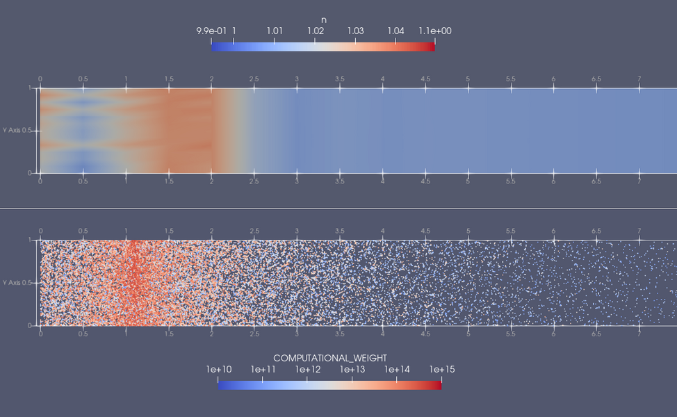
Zoom-in on one end of the 2D domain showing the plasma number density (top) and distribution of neutral particles (bottom) coloured by weight.
Running a solver#
While each solver executable can be used directly, the simplest way to run a solver example is using the run_eg.sh script.
This ensures all required input files are copied to a new directory (runs/<solver_name>/<examples_name>) and that the correct command is executed.
To run the script from the repository root, use:
- Usage:
./scripts/run_eg.sh [solver_name] [example_name] <-n num_MPI> <-b build_dir/install_dir>
Note that the number of MPI processes can be set via a command line flag, and defaults to 4.
The script assumes the intended mpirun executable is on your path and looks for solver executables in the most recently modified spack “view” directory.
To use a different solver executable, supply the build directory or install directory as described.
Caution: When running with (MPI and) OpenMP, a value must be set for the OMP_NUM_THREADS environment variable. If OMP_NUM_THREADS isn’t set, the number of threads will be chosen automatically, typically resulting in one thread per logical core. This often leads to oversubscription of cores and slow simulations. It usually makes sense to execute
export OMP_NUM_THREADS=1
before running an example.
Modifying example meshes#
All examples in the repository include a Nektar++-compatible XML mesh.
Users that wish to modify those meshes, or create new ones for other applications can use geo_to_xml.sh.
The script takes a .geo file as input, and uses gmsh and NekMesh to convert it to .xml.
To run the script from the repository root, use:
- Usage:
- ./scripts/geo_to_xml.sh [path_to_geo_file] <options>
- Options include
Specifying a path and/or arguments for gmsh: <-g gmsh_path> <–gmsh_args “arg1 arg2…”>
Specifying a path and/or XML file properties for NekMesh: <-m NekMesh_path> <-p “prop1 prop2…”> (e.g. -p “uncompress” to generate a human-readable, uncompressed XML file)
Setting an output filename <-o output_filename>
Specifying composite IDs for periodic boundary conditions <-x x_bndry_compIDs> <-y y_bndry_compIDs> <-z z_bndry_compIDs> (e.g. -x 1,2 -y 3,4 -z 5,6)
Both gmsh and NekMesh are expected to be on the path.
Note that, if NESO was installed with spack, then NekMesh should already be built.
Run
spack find -l nektar
to see which versions of Nektar++ are available, along with their 7-digit hashes, then
export PATH=$PATH:$(spack location -i nektar/[hash])/bin
to add the Nektar++ binaries, including NekMesh, to your path.