Software Engineering Response

The above scientific response Section 4.1 indicates that the NEPTUNE suite will have the capability to describe the tokamak edge in a comprehensive set of levels of detail using a large range of possibly heterogeneous computer hardware, will be straightforwardly modifiable to include additional physical effects, and will aim to include under all circumstances, the level of error in computed results. Evidently, eveloping the suite represents a major challenge to current software engineering practices thanks to its scientific difficulty as indicated in Section 4.A, and perhaps less obviously, its scientific complexity due to the need to treat large numbers of atomic and molecular species, descending to the level of isotopes with a range of charge states and electronic excitations.

The last makes NEPTUNE a significantly harder development than the BOUT++ code discussed in Section 4.1. The difficulty motivated studies of software engineering practices outside as well as in the scientific context. The studies of scientific work are summarised in reports concerning frameworks, scientific UQ etc. Ideas from these studies are combined with non-technical works such as Hewitt ref. [28] and Sommerville ref. [29] and summarised in the report ref. [2].

The outcome is the present report and website, which augment the procedures of Dudson and BOUT++ collaborators ref. [3] to govern the development of NEPTUNE. Management aspects of the development are treated in Section 7.1 and operational aspects in Section 9.1. The remainder of this section focusses on the generic details of a software implementation, the so-called non-functional aspects, with BOUT++ instructions augmented to allow for the greater complexity of NEPTUNE, following the D3.3 reports ref. [30], here with Section 4.3 adding a way to handle a multitude of variable names to accommodate the much increased number of physical variables.

Following D3.3 ref. [30], Section 4.2 discusses high-level constraints on the structure of software. where the concept of division into packages and modules (which may represent libraries) is promoted. Section 4.2 explores the implications of these constraints for NEPTUNE. At the opposite extreme to Section 4.2 and Section 4.2, Section 4.2 describes the desirable contents for a single module, and Section 4.2 discusses the question of what best to output when developing software for the Exascale.

General Considerations

It is important that individual units of code are manageable and the overall structure is comprehensible, so that developers and users can navigate the codebase and determine where new work is to be located. This simple consideration implies that NEPTUNE software should be divided into units that it will be convenient to refer to as modules, ie. sections of code containing everything necessary to perform one (and only one) aspect of the desired functionality.

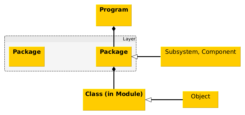
The suggested content of a module describing a single class in the UML sense (see Section 4.2, Table 4.1) implies a minimum of \(13\) methods described by separate subroutines/functions, with examples extending up to \(50\), although the latter is there regarded as an excessively large number of methods. Many small software libraries also fall into this size range. Supposing that each subroutine is of a length to fit within one computer window, ie. up to about \(60\) lines, the desirable maximum length of a well-designed module file is \(30\times 60 = 1\,800\) lines which is a manageable size of file given editing software that remembers on restart, the last line accessed (so that it possible to return immediately to a particular subroutine). The magnitude of the D3.3 exercise follows from the fact that comparable software packages probably of somewhat lesser complexity than NEPTUNE written in high level languages such as C++ range in size up to \(1\,000\,000\) lines. Clearly \(400\) separate modules is too unwieldy, and there is a need to organise further into packages which might contain in turn \(10\)-\(50\) modules. As a way of providing further indication to developers, it is helpful to talk of packages as being arranged into layers, as discussed in ref. [31, §§ 2.4, 3.2], see Figure 4.4. Then, as prefigured in ref. [31, Annex A], it should be possible to encapsulate the necessary complexity in one, albeit large diagram.

Considerations for Scientific Software

Structural Considerations

In both refs. [32, 33], a figure from Dubey et al ref. [34] is reproduced that illustrates how scientific software may be developed by beginning with an “infrastructure" capability into which initially exploratory scientific software is integrated as its worth is established. Unfortunately for NEPTUNE, it is not clear initially what aspects of the infrastructure will be durable and stable, although once the software is more mature, Dubey et al’s methodology appears attractive.

The literature referenced in ref. [31] indicates that scientific software should be produced by aggregation, but is less helpful as to what is to be aggregated, ie. the modular decomposition as to what should constitute a single module etc.

Since the NEPTUNE development will proceed as a series of proxyapps, there is a chance to refine and redefine an initial modular decomposition with each successive proxyapp, recording the results as a UML structure diagram. When generating the corresponding sequence diagram (ie. procedural description), the proxyapp-based units should be preserved to facilitate the use of the simpler ones as surrogates for the later more complex proxyapps.

To help understand the aggregation of the software, it should be layered in the obvious manner, with the higher layers corresponding to greater numbers of aggregated objects. It is also expected to be useful to classify the modules. The modules should be arranged into a relatively small number of packages according to, eg. whether they treat particle generation, matrix coefficient calculation, the main matrix solution, or visualisation.

Interactions between Modules

Concerning logical interconnections between modules, the use of a directed, acyclic graph (DAG) structure might be thought mandatory, particularly to process the input data in order to specify coherently the construction of the elements of the solution matrix. However, as prefigured in ref. [31] for the gyrokinetics code GS2, the tightly coupled nature of the central edge physics problem means that input is more about gathering all the data, for only at that point can fields be computed and only after that may matrix coefficients be computed.

(TODO) “Information hiding principle" eg. input data module “hides" information about how this is done from the calculation module: it just passes along parameters in an agreed format. Can extend this idea on to every level - eg. Parnas advocates hiding the hardware from the code - cf. performance portability. Such modularity enables work to be efficiently assigned to a programmer or group.

Design of a Module

Notation

UML nomenclature is preferred herein, for which Table 4.1 provides a limited translation into C++ and Object Fortran.

Module design

The focus herein is the structure within a module. Specifically, the module describes a single class or object (strictly speaking in UML terms, objects are instances of a class), which is fundamental in that it is defined without use of aggregation. The software - consistent with Clerman and Spector ref. [35, § 11] - that is promoted by Arter et al ref. [36] for an object-oriented language, recognises two sizes of fundamental class and it is easier to start by considering the smaller, denoted smallobj_m.

Module smallobj_m does not have a separate attributes file, but will typically still use or access three or more yet more fundamental classes, namely

• • log_m for logging errors or warnings in code execution, and checkpointing values of selected variables

• • const_numphys_h for numerical values of important mathematical and physical constants relevant to plasma physics

• • const_kind_m to specify precision of representation of real and integer values, together with formatting to be used for their output (in fact contains no executable code)

• • date_time_m to return the date and time in either a verbose or minimal format

• • misc_m to form miscellaneous operations found to be common to many modules

In outline, the methods or operations associated with smallobj allow data to be read from a named file, used in the construction of an object, and output to disc file. The file is given a numeric identifier ninso (file unit) when it is opened. Data used to construct the object forms a single namelist block, viz. a list of arbitrary code variables that may (or not) be assigned values in the input file using a attribute-value notation. Namelist variables should have long names that promote a good user interface, and be given default values in case they are not input. The style encourages checking that inputs have acceptable values, for example lie in expected ranges, but there is no equivalent of eg. the Cerberus Python data validation package ref. [37], users must explicitly code checks and calls to log_m if the values are questionable or erroneous. (It is hoped that this can be automated based on a LaTeX table describing input symbols. After successful checks, the values in the namelist are copied into the data type sonumerics_t, whence it is supposed that a single subroutine then instantiates the smallobj_t object. Another routine performs output of this object, either to a directly specified file unit, or to the standard output by default, in the simple text format of a variable name followed by its value on the following line. As might be expected, there are also routines to ‘delete’ the object, ie. to deallocate any constituent arrays, and to close the input file. The precise list of member functions (or methods in the UML nomenclature) is

• • initfile, open input file

• • readcon, read data from input file

• • generic, generic subroutine to instantiate object

• • write, write out object to standard output, or to file opened by another object

• • delete, delete object

• • close, close input file

Module bigobj_m has a separate file for its attributes (aka namespace), which it will normally still use or access like the yet more fundamental objects listed for smallobj_m. However the data types defined in bigobj_h are of the same kind as those in smallobj_m, viz. bonumerics_t to hold input data which is used to define bigobj_t by calling the solve subroutine (rather than the subroutine generic in the case of smallobj_m). Apart from this last exception, the methods in bigobj_m are a superset of those in smallobj_m. The additional methods recognise that instantiation may involve more than one routine and in particular may involve use of a specially defined function fn, demonstrating the STRATEGY Pattern or possibly TEMPLATE Pattern. This function may be determined by a formula identified in the input, giving the option for a developer or determined user of adding their own code to define a new function. The range of allowable outputs is much extended. Thus there is a separate routine provided for output to the log file using what will probably be a lengthy list of calls to log_value_m. More likely to be useful is a routine to open an .out file on a file unit given the number noutbo on opening, which becomes the default unit for writing out the object in bigobj_write. There are also provided separate skeleton routines intended to provide output in a format suitable respectively for visualisation by gnuplot and ParaView, and of course routines to close files and delete the object. The precise list of member functions for bigobj_m is as follows where those also found in smallobj_m are enclosed in parenthesis:

• • (initfile), open input file

• • (readcon), read data from input file

• • solve, generic subroutine to manage instantiation of object

• • userdefined, user-defined method or function

• • fn, general external function call

• • dia, write object diagnostics to log file

• • initwrite, open new file, making up name which defaults to having .out suffix

• • (write), write out object to standard output, or to file opened by bigobj

• • writeg, write out object suitable for visualisation by gnuplot

• • writev, write out object suitable for visualisation by ParaView

• • (delete), delete object

• • (close), close input file

• • closewrite, close write file opened by initwrite

Thus the skeleton object is defined by a formula plus data input from disc, and since both are saved internally as features, the instantiation may be deferred as necessary, so-called ‘lazy initialisation’. It will be noticed that other variables in bigobj_m such as unit number are hidden, ie. cannot be accessed by other modules. In fact a common addition to the default modules is a method function getunit that returns ninbo, illustrating the approved way of accessing such data.

The reason for the emphasis on input and output from and to disc (I/O) is to facilitate the construction of a test harness for an objects in the style of bigobj_m, and indeed the aggregations of such objects. The use of “attribute-value" in I/O gives flexibility to the developer, since new variables may be added without the need to modify existing input files or output processing. Output processing is further discussed in Section 4.2.

Processing Module Output

The number of I/O subroutines can be criticised. For many testing purposes an interactive debugger is adequate, and for most others that one output file is sufficient provided it is in a attribute-value format such as JavaScript Object Notation (JSON) or in a self-documenting format such as the Network Common Data Form (netCDF), to be interpreted by any suitable visualisation software.

The problem with scientific software, worse at Exascale, is the volume of data to be handled so that the ability to visualise large arrays as well as large numbers of small arrays is essential (no debugger as far as is known has such a visualisation feature). Moreover, the actionable aspect of NEPTUNE further means that any postprocessing of a generic file must also be carefully performed. Thus while a generic output file could be processed by say Linux awk script into a form suitable for gnuplot processing, this gives rise to a need for providing documentation and provenance for the script, which is at minimum a nuisance. Worse is the risk that the amount of data to be processed may be so large as to lead to significant delay and maybe even system or other issues not handled well if at all by the script, all of which may be extremely time-consuming to resolve. Other conversion software may not be available or properly implemented on the target machine. Thus even for debugging purposes, it seems desirable that as much as possible of the processing is done within the main code, and for production runs, output in a format directly readable by say ParaView should also speed the post-processing. Since netCDF may be read directly by ParaView, this is recommended.

Code licence and availability

Code should be made available to collaborators at the earliest opportunity, to maintain close alignment between groups.

• • To minimise friction and unnecessary legal restrictions on combining code components, a common, MIT licence has been adopted. This may be regarded as equivalent to the BSD3 licence in the NEPTUNE Charter, see Section 7.3.

• • Code development should be carried out in public repositories. The benefits of minimising delay to code use, feedback and peer review, outweigh any potential for embarrassment or code misuse.

Code style

There are many different code styles, each of which have their proponents, and can be debated at length. While everyone has their own favourite style, it seems likely that the choice of style makes little difference to objective quality or productivity. Anecdotal experience and experience from the gaming world in developing large, complicated packages (eg. Gregory ref. [38, § 3]), indicate however that it is very important that there is a well-defined code style and that developers stick to it, since a mixture of styles in a code base adds unnecessary mental load and overhead. The ultimate choice is down to the project Lead, under advice from major code contributors, leading websites and textbooks, eg. in the case of the C++ language, the C++ core guidelines ref. [39] and more compactly Stroustrop’s “Tour of of C++" ref. [40].

The following style choices have been made and efforts will be made to enforce them in NEPTUNE repositories.

• 1. Formatting of C++ and Python will follow the style used by Nektar++

  • • Developer tools: Code formatting tools should be used to automatically format code. For C++ clang-tidy ref. [41] should be used while, and for Python Black ref. [42] is recommended. Similar tools should be chosen for any other languages adopted by the project.

  • • Enforcement: Tests run on pull requests and code pushes to the shared repository should include code formatting: The automated formatter is applied to the code, and if the output is different from the input then the code is incorrectly formatted, and the test fails.

  • • Documentation: LaTeX or Markdown should be used and conventions enforced regarding a maximum line length of \(120\) characters, restriction to ASCII character set, abbreviations, hyphenation, capitalisation, minimal use of ‘z’, and use of fonts to denote code names. The LaTeX lwarp package is used to generate this website.

• 2. Naming

  Naming of code components (modules, classes, functions, variables etc.) is less easy to enforce automatically than formatting, but is arguably essential for NEPTUNE, because of the complexity of the physical processes to be modelled. Widely applicable good practices to be adopted are as follows:

  • • Consistency: Whatever convention is used, stick to it.

  • • Be descriptive: Names should be meaningful, not cryptic, and need not be very short, although brevity consistent with frequency of usage is recommended.

    • – Variable names, used only on input, might consist of \(3-4\) words primarily describing the variable, using ‘pot-hole’ convention

    • – Loop or indexing variables, might consist of single characters, eg. i, j, k

    • – Mathematical symbols, eg. those defined in Section 11.3, should be converted from LaTeX into variable names using the conventions of Section 11.1.

    • – Where mathematical symbols are converted for use in larger expressions, the mathematical expression should be in the documentation within or linked to the code.

  • • Generally prefer nouns for variables, and verbs for functions

  Given a need to mix with Object Fortran, which is not case-sensitive, the ‘pot-hole’ convention for naming C++ variables, ie. separating name elements by underscores, is recommended.

  Occasionally a convention is used where the name includes a part which indicates the type of the variable. For example, the JSF style for C++ ref. [43, § 6.6] recommends that pointer names begin ‘p_’ and that private or protected (‘member’) variables should have names beginning with ‘m’. In general naming conventions are probably not essential, since the type can be read in the code, and modern IDEs will easily provide this information to the developer. Nonetheless, there is no objection to employing a convention, and NEPTUNE recommend the following one for coders who wish to do so.

  For C++, based on the recommendations of the book “Professional C++" (eg. ref. [44, § 7], the following prefix strings should be employed: ‘m_’ for member (particularly useful for indicating scope), ‘p_’ for pointer, ‘s_’ for static, ‘k_’ for constant, ‘f_’ for flag (Boolean value), ‘d_’ for buffers/pointers on an accelerator device, and aggregations thereof, eg. ‘ms_variable’. Use of global variables is deprecated, so the ‘g_’ prefix should not be used.

  For Object Fortran naming conventions, Arter et al ref. [36] codifies best practice. It may also be useful to reserve the single letters ‘i’, ‘j’, ‘k’ etc. for the names of loop-count variables. Loop counting should start at unity, consistent with everyday practice, unless there are good reasons for starting at zero or using offset values.

Programming languages

A small set of “approved" languages is to be used in the project consistent with the rule of ‘two’ described in Section 7.1. This rule covers the high performance code itself and also the input/output, testing scripts and other infrastructure included in the code repository.

Important factors in the choice made included:

• 1. Widespread use. It must be possible for several project members at any one time to understand the language, and be able to maintain the code.

• 2. Stability. The code developed will potentially have a long life-span, and there are insufficient resources to continually update code to respond to upstream changes.

• 3. Previous usage in HPC and scientific computing. There should be an existing ecosystem of code packages, tutorials, and potential users.

The above considerations implied that the following options were extensively discussed.

• • C++14, Fortran (eg. 2008), C and Python all satisfy the above criteria. For configuration, CMake, Autotools and Bash also qualify.

• • SYCL (building on C++) and Julia are both less widely adopted so far, but both appear to be heading towards satisfying the above criteria and might be considered.

The recommended languages are

• • As higher level DSL : Python and Julia

• • For lower level HPC compatibility/DSL: Kokkos and SYCL

• • General scientific work : the latest versions of C++ and (Object) Fortran, provided they are compatible with pre-existing packages and reliable compilers are available (eg. as of mid-2021 usage of SYCL implies a need for C++17.)

• • For code compilation and linking etc. : CMake

Other languages may have technical merits in particular areas, or are being adopted outside scientific computing but not to a significant degree within the community. Use of these languages should be limited to isolated experiments, rather than core components. If shown to be useful in these experiments, to a level which is worth the additional overhead and risk of maintaining it, then the Lead should consider expanding the list of approved languages, consistent with the ‘rule of two’.